If you haven’t read the previous parts of this series yet, here are the links: [ Part 1 | Part 2 ].
A Refresher
In the first part of this series I said that RAM access is the slow component of a modern in-memory database engine and for performance you’d want to reduce RAM access as much as possible. Reduced memory traffic thanks to the new columnar data formats is the most important enabler for the awesome In-Memory processing performance and SIMD is just icing on the cake.
In the second part I also showed how to measure the CPU efficiency of your (Oracle) process using a Linux perf stat command. How well your applications actually utilize your CPU execution units depends on many factors. The biggest factor is your process’es cache efficiency that depends on the CPU cache size and your application’s memory access patterns. Regardless of what the OS CPU accounting tools like top or vmstat may show you, your “100% busy” CPUs may actually spend a significant amount of their cycles internally idle, with a stalled pipeline, waiting for some event (like a memory line arrival from RAM) to happen.
Luckily there are plenty of tools for measuring what’s actually going on inside the CPUs, thanks to modern processors having CPU Performance Counters (CPC) built in to them.
A key derived metric for understanding CPU-efficiency is the IPC (instructions per cycle). Years ago people were actually talking about the inverse metric CPI (cycles per instruction) as on average it took more than one CPU cycle to complete an instruction’s execution (again, due to the abovementioned reasons like memory stalls). However, thanks to today’s superscalar processors with out-of-order execution on a modern CPU’s multiple execution units – and with large CPU caches – a well-optimized application can execute multiple instructions per a single CPU cycle, thus it’s more natural to use the IPC (instructions-per-cycle) metric. With IPC, higher is better.
Here’s a trimmed snippet from the previous article, a process that was doing a fully cached full table scan of an Oracle table (stored in plain old row-oriented format):
Performance counter stats for process id '34783':

      27373.819908 task-clock                #    0.912 CPUs utilized
    86,428,653,040 cycles                    #    3.157 GHz                     [33.33%]
    32,115,412,877 instructions              #    0.37  insns per cycle
                                             #    2.39  stalled cycles per insn [40.00%]
    76,697,049,420 stalled-cycles-frontend   #   88.74% frontend cycles idle    [40.00%]
    58,627,393,395 stalled-cycles-backend    #   67.83% backend  cycles idle    [40.00%]
       256,440,384 cache-references          #    9.368 M/sec                   [26.67%]
       222,036,981 cache-misses              #   86.584 % of all cache refs     [26.66%]

      30.000601214 seconds time elapsed
The IPC of the above task is pretty bad – the CPU managed to complete only 0.37 instructions per CPU cycle. On average every instruction execution was stalled in the execution pipeline for 2.39 CPU cycles.
Note: Various additional metrics can be used for drilling down into why the CPUs spent so much time stalling (like cache misses & RAM access). I covered the typical perf stat metrics in the part 2 of this series so won’t go in more detail here.
Test Scenarios
The goal of my experiments was to measure the number CPU-efficiency of different data scanning approaches in Oracle – on different data storage formats. I focused only on data scanning and filtering, not joins or aggregations. I ensured that everything would be cached in Oracle’s buffer cache or in-memory column store for all test runs – so disk IO was not a factor here (again, read more about my test environment setup in part 2 of this series).
The queries I ran were mostly variations of this:
SELECT COUNT(cust_valid) FROM customers_nopart c WHERE cust_id > 0
Although I was after testing the full table scanning speeds, I also added two examples of scanning through the entire table’s rows via index range scans. This allows me to show how inefficient index range scans can be when accessing a large part of a table’s rows even when all is cached in memory. Even though you see different WHERE clauses in some of the tests, they all are designed so that they go through all rows of the table (just using different access patterns and code paths).
The descriptions of test runs should be self-explanatory:
1. INDEX RANGE SCAN BAD CLUSTERING FACTOR
SELECT /*+ MONITOR INDEX(c(cust_postal_code)) */ COUNT(cust_valid)
FROM customers_nopart c WHERE cust_postal_code > '0';
2. INDEX RANGE SCAN GOOD CLUSTERING FACTOR
SELECT /*+ MONITOR INDEX(c(cust_id)) */ COUNT(cust_valid)
FROM customers_nopart c WHERE cust_id > 0;
3. FULL TABLE SCAN BUFFER CACHE (NO INMEMORY)
SELECT /*+ MONITOR FULL(c) NO_INMEMORY */ COUNT(cust_valid)
FROM customers_nopart c WHERE cust_id > 0;
4. FULL TABLE SCAN IN MEMORY WITH WHERE cust_id > 0
SELECT /*+ MONITOR FULL(c) INMEMORY */ COUNT(cust_valid)
FROM customers_nopart c WHERE cust_id > 0;
5. FULL TABLE SCAN IN MEMORY WITHOUT WHERE CLAUSE
SELECT /*+ MONITOR FULL(c) INMEMORY */ COUNT(cust_valid)
FROM customers_nopart c;
6. FULL TABLE SCAN VIA BUFFER CACHE OF HCC QUERY LOW COLUMNAR-COMPRESSED TABLE
SELECT /*+ MONITOR */ COUNT(cust_valid)
FROM customers_nopart_hcc_ql WHERE cust_id > 0
Note how all experiments except the last one are scanning the same physical table just with different options (like index scan or in-memory access path) enabled. The last experiment is against a copy of the same table (same columns, same rows), but just physically formatted in the HCC format (and fully cached in buffer cache).
Test Results: Raw Numbers
It is not enough to just look into the CPU performance counters of different experiments, they are too low level. For the full picture, we also want to know how much work (like logical IOs etc) the application was doing and how many rows were eventually processed in each case. Also I verified that I did get the exact desired execution plans, access paths and that no physical IOs or other wait events happened using the usual Oracle metrics (see the log below).
Here’s the experiment log file with full performance numbers from SQL Monitoring reports, Snapper and perf stat:
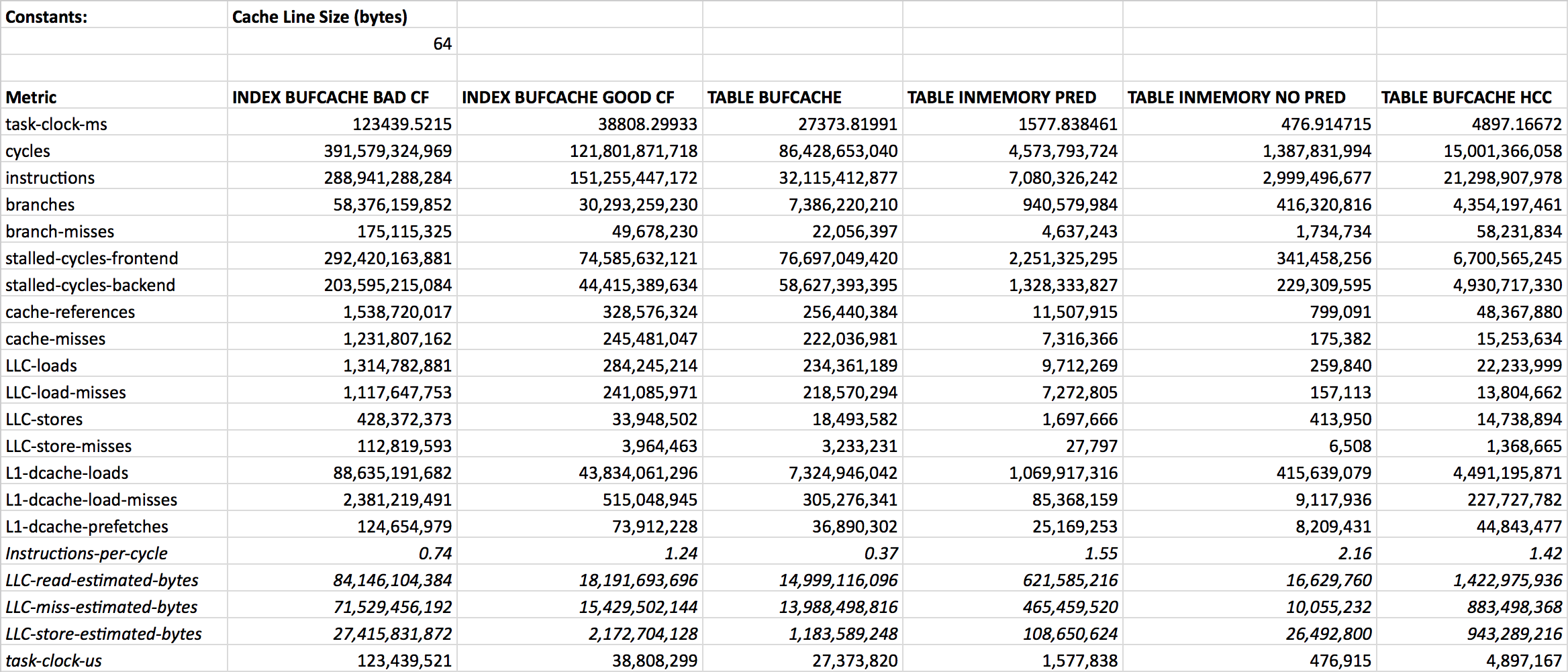
I also put all these numbers (plus some derived values) into a spreadsheet. I’ve pasted a screenshot of the data below for convenience, but you can access the entire spreadsheet with its raw data and charts here (note that the spreadsheet has multiple tabs and configurable pivot charts in it):
- https://docs.google.com/spreadsheets/d/1ss0rBG8mePAVYP4hlpvjqAAlHnZqmuVmSFbHMLDsjaU/edit?usp=sharing
Raw perf stat data from the experiments:
Now let’s plot some charts!
Test Results: CPU Instructions
Let’s start from something simple and gradually work our way deeper. I will start from listing the task-clock-ms metric that shows the CPU time usage of the Oracle process in milliseconds for each of my test table scans. This metric comes from the OS-level and not from within the CPU:
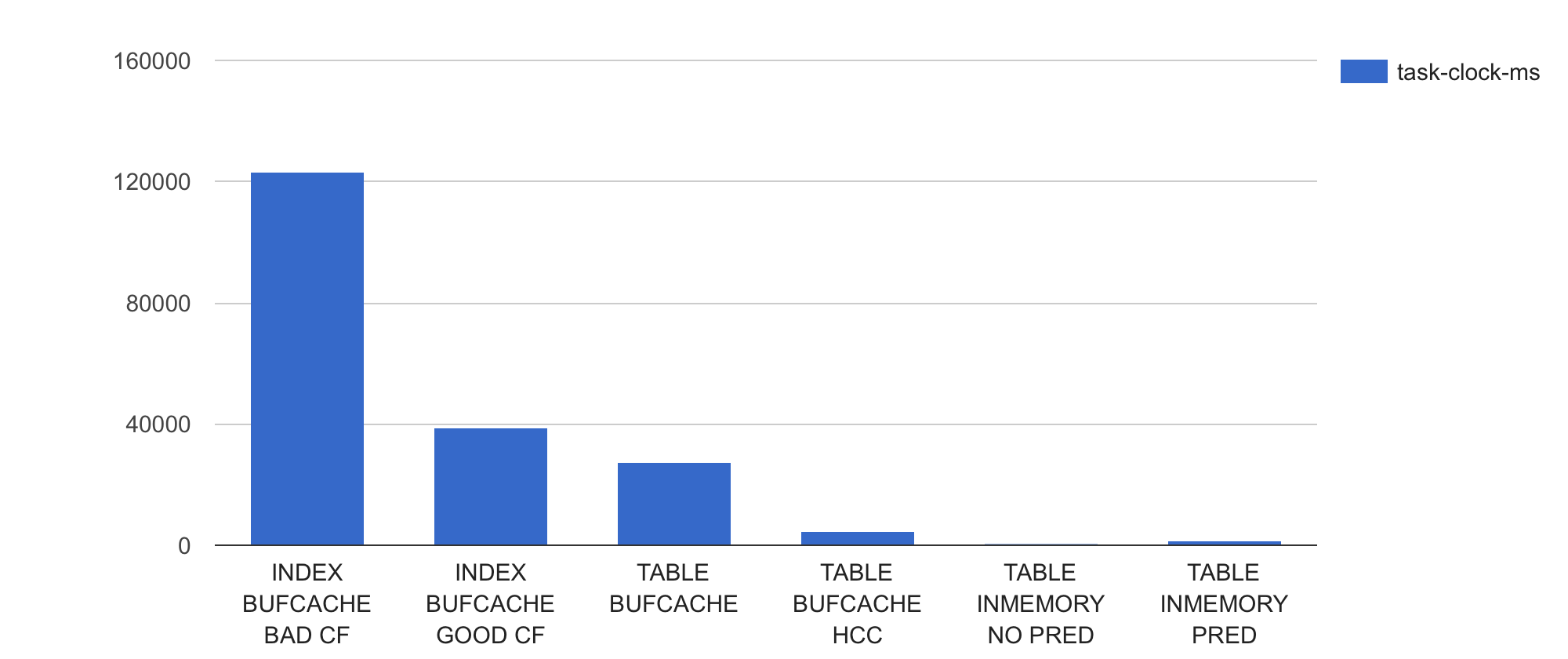
As I mentioned earlier, I added two index (full) range scan based approaches for comparison. Looks like the index-based “full table scans” seen in first and second columns are using the most CPU-time as the OS sees it (~120 and close to 40 seconds of CPU respectively).
Now let’s see how many CPU instructions (how much work “requested” from CPU) the Oracle process executed for scanning the same dataset using different access paths and storage formats:
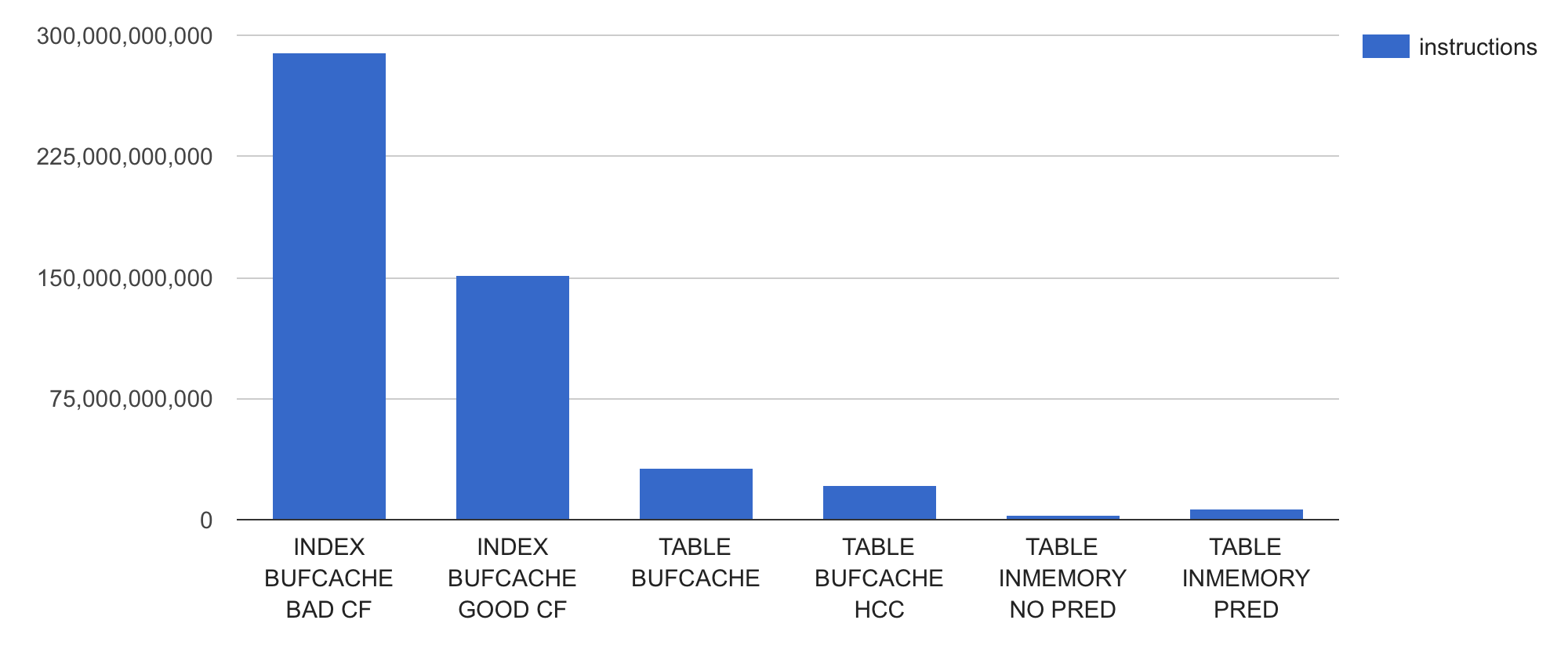
Wow, the index-based approaches seem to be issuing multiple times more CPU instructions per query execution than any of the full table scans. Whatever loops the Oracle process is executing for processing the index-based query, it runs more of them. Or whatever functions it calls within those loops, the functions are “fatter”. Or both.
Let’s look into an Oracle-level metric session logical reads to see how many buffer gets it is doing:
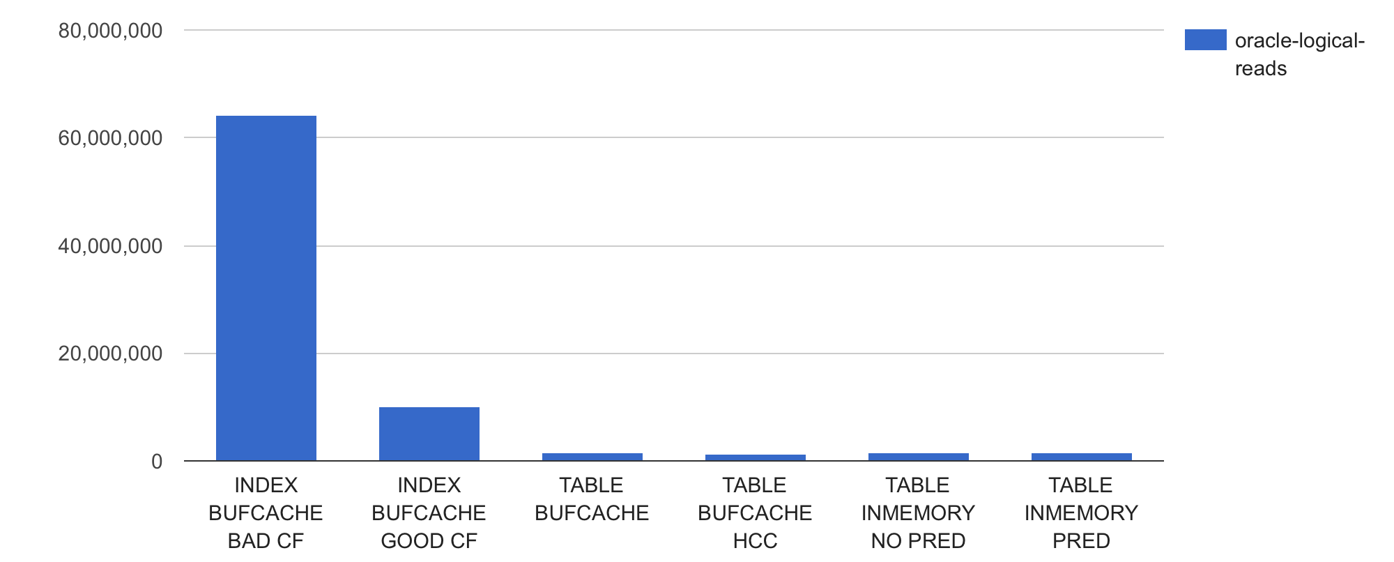
Wow, using the index with bad clustering factor (1st bar) causes Oracle to do over 60M logical IOs, while the table scans do around 1.6M of logical IOs each. Retrieving all rows of a table via an index range scan is super-inefficient, given that the underlying table size is only 1613824 blocks.
This inefficiency is due to index range scans having to re-visit the same datablocks multiple times (up to one visit per row, depending on the clustering factor of the index used). This would cause another logical IO and use more CPU cycles for each buffer re-visit, except in cases where Oracle has managed to keep a buffer pinned since last visit. The index range scan with a good clustering factor needs to do much fewer logical IOs as given the more “local” clustered table access pattern, the re-visited buffers are much more likely found already looked-up and pinned (shown as the buffer is pinned count metric in V$SESSTAT).
Knowing that my test table has 69,642,625 rows in it, I can also derive an average CPU instructions per row processed metric from the total instruction amounts:
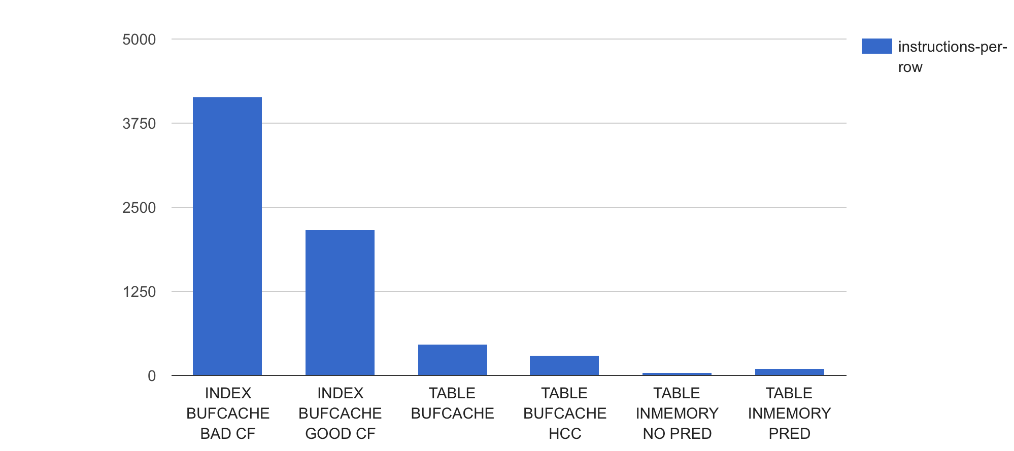
The same numbers in tabular form:
Indeed there seem to be radical code path differences (that come from underlying data and cache structure differences) that make an index-based lookup use thousands of instructions per row processed, while an in-memory scan with a single predicate used only 102 instructions per row processed on average. The in-memory counting without any predicates didn’t need to execute any data comparison logic in it, so could do its data access and counting with only 43 instructions per row on average.
So far I’ve shown you some basic stuff. As this article is about studying the full table scan efficiency, I will omit the index-access metrics from further charts. The raw metrics are all available in the raw text file and spreadsheet mentioned above.
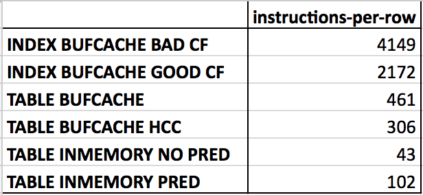
Here are again the buffer gets of only the four different full table scan test cases:
All test cases except the HCC-compressed table scan cause the same amount of buffer gets (~1.6M) as this is the original table’s size in blocks. The HCC table is only slightly smaller – didn’t get great compression with the query low setting.
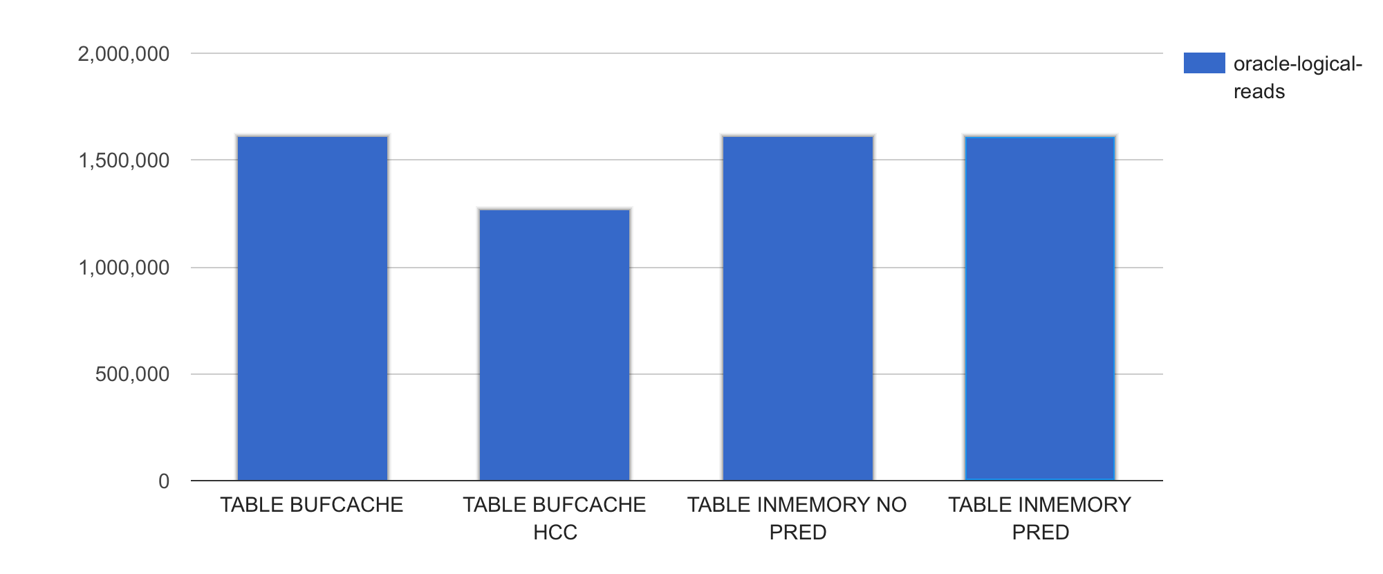
Now let’s check the number CPU instructions executed by these test runs:
Wow, despite the table sizes and number of logical IOs being relatively similar, the amount of machine code the Oracle process executes is wildly different! Remember, all that my query is doing is just scanning and filtering the data followed with a basic COUNT(column) operation – no additional sorting, joining is done. The in-memory access paths (column 3 & 4) get away with executing much fewer CPU instructions than the regular buffered tables in row-format and HCC format (columns 1 & 2 in the chart).
All the above shows that not all logical IOs are equal, depending on your workload and execution plans (how many block visits, how many rows extracted per block visit) and underlying storage formats (regular row-format, HCC in buffer cache or compressed columns in In-Memory column store), you may end up doing a different amount of CPU work per row retrieved for your query.
This was true before the In-Memory option and even more noticeable with the In-Memory option. But more about this in a future article.
Test Results: CPU Cycles
Let’s go deeper. We already looked into how many buffer gets and CPU instructions the process executed for the different test cases. Now let’s look into how much actual CPU time (in form of CPU cycles) these tests consumed. I added the CPU cycles metric to instructions for that:
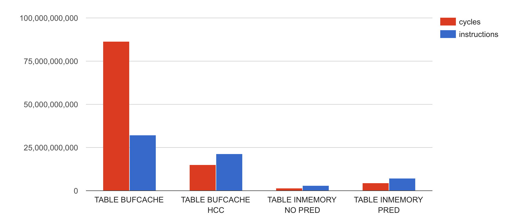
Hey, what? How come the regular row-oriented block format table scan (TABLE BUFCACHE) takes over twice more CPU cycles compared to its instructions executed?
Also, how come all the other table access methods use noticeably less CPU cycles than the number of instructions they’ve executed?
If you paid attention to this article (and previous ones) you’ll already know why. In the 1st example (TABLE BUFCACHE) the CPU must have been “waiting” for something a lot, instructions having spent multiple cycles “idle”, stalled in the pipeline, waiting for some event or necessary condition to happen (like a memory line arriving from RAM).
For example, if you are constantly waiting for the “random” RAM lines you want to access due to inefficient memory structures for scanning (like Oracle’s row-oriented datablocks), the CPU will be bottlenecked by RAM access. The CPU’s internal execution units, other than the load-store units, would be idle most of the time. The OS top command would still show you 100% utilization of a CPU by your process, but in reality you could squeeze much more out of your CPU if it didn’t have to wait for RAM so much.
In the other 3 examples above (columns 2-4), apparently there is no serious RAM (or other pipeline-stalling) bottleneck as in all cases we are able to use the multiple execution units of modern superscalar CPUs to complete more than one instruction per CPU cycle. Of course more improvements might be possible, but more about this in a following post.
For now I’ll conclude this (lengthy) post with one more chart with the fundamental derived metric instructions per cycle (IPC):
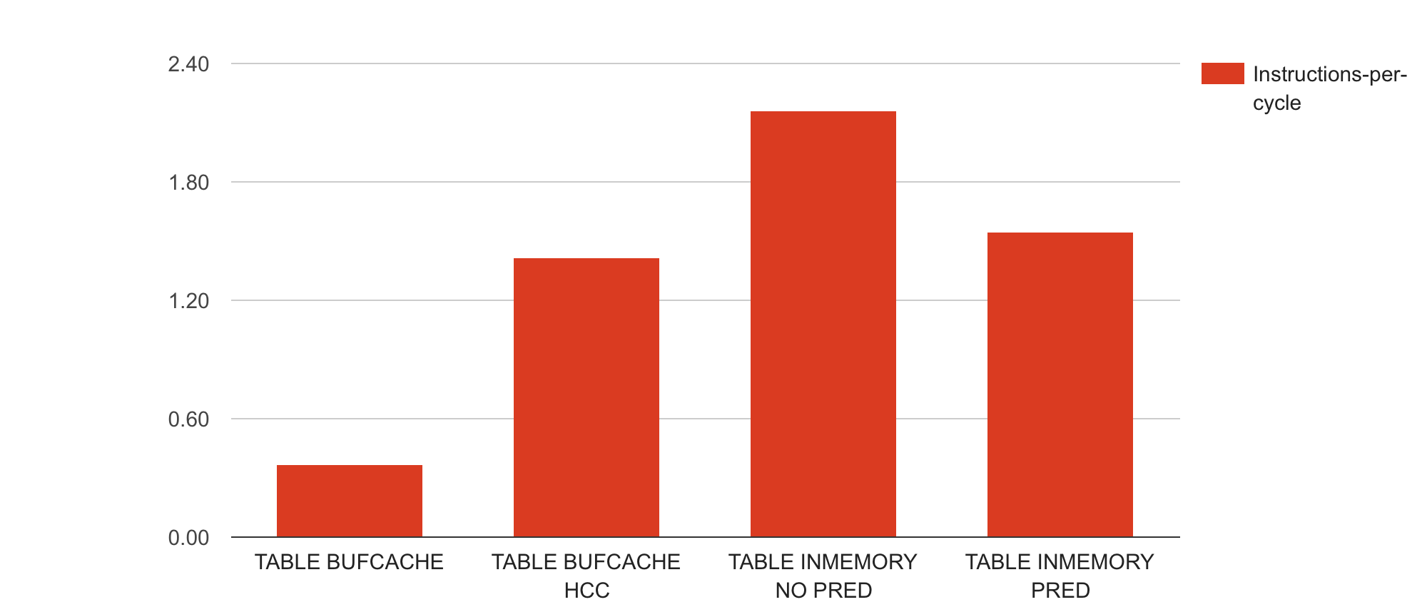
The IPC metric is derived from the previously shown instructions and CPU cycles metrics by a simple division. Higher IPC is better as it means that your CPU execution units are more utilized, it gets more done. However, as IPC is a ratio, you should never look into the IPC value alone, always look into it together with instructions and cycles metrics. It’s better to execute 1 Million instructions with IPC of 0.5 than 1 Billion instructions with an IPC of 3 – but looking into IPC in isolation doesn’t tell you how much work was actually done. Additionally, you’d want to use your application level metrics that give you an indication of how much application work got done (I used Oracle’s buffer gets and rows processed metrics for this).
Looks like there’s at least 2 more parts left in this series (advanced metrics and a summary), but let’s see how it goes. Sorry for any typos, it’s getting quite late and I’ll fix ’em some other day :)
Discussion & Further reading
- There are some additional comments in HackerNews
- Check out my my open source 0x.tools toolset - Always on Profiling for Linux Production Systems